Summary of the Catenary
The catenary curve is graphed as $$f(x)=a\cosh\left(\frac{x}{a}\right).\tag{CS-1} \label{CS-1}$$ This is true whether there are equal or unequal height attachment points. The $y$-axis will pass through the lowest point of the curve, assuming $a$ is positive. Value $a$ is sometimes called the catenary constant. It is the distance from the graph origin to the low point of the curve. If we want to bring the curve down to the $x$-axis we write $$f(x)=a\cosh\left(\frac{x}{a}\right)-a \tag{CS-2} \label{CS-2} $$
The tension equations are $$T_{0}=T\cos\theta \tag{CS-3} \label{CS-3}$$ and $$\omega_{0}s=T\sin\theta \tag{CS-4} \label{CS-4}$$ $\omega_{0}$ is the weight/length of the cable and we defined $$a=\frac{T_{0}}{\omega_{0}} \tag{CS-5} \label{CS-5}$$ When $s$ is the length of some cable section, we found that $$\frac{s}{a}=\sinh\left(\frac{x}{a}\right). \tag{CS-6} \label{6}$$ This is easily solved for $x.$ $$x=a\sinh^{-1}\left(\frac{s}{a}\right) \tag{CS-7} \label{CS-7}$$ $x$ is always the horizontal distance from the $y$-axis to the attachment. We defined $h$ to be the vertical distance from an attachment to the low point of the curve. If the attachments were at different heights, then we had an $h_{1}$ and $h_{2}.$ Since equation $\eqref{CS-2}$ moved the curve down to the x-axis, $$f(x)=h=a\cosh\left(\frac{x}{a}\right)-a. \tag{CS-8} \label{CS-8}$$ The derivative of $\eqref{CS-1}$ is $$\frac{df(x)}{dx}=\sinh\left(\frac{x}{a}\right) \tag{CS-9} \label{9}$$ but $$\frac{df(x)}{dx}=\tan\theta \tag{CS-10} \label{CS-10}$$ and $$\theta=\tan^{-1}\left(\sinh\left(\frac{x}{a}\right)\right). \tag{CS-11} \label{CS-11}$$ It is often useful to look at $\theta$ at an attachment point. When general information is given about tension, $T_{0}$ is the tension given. That way, $T_{0}=\omega_{0}a$ gives up the catenary constant $a$ and everything else follows. Also, at low angles, $T=T_{0}.$
To find catenary constant, $a$, when sag, $h$, and distance $x$ are given: $$f(a)=a\cosh\left(\frac{x}{a}\right)-a-h$$ $$f^{\prime}(a)=-x\frac{\sinh\left(\frac{x}{a}\right)}{a}+\cosh\left(\frac{x}{a}\right)-1$$ $$a_{new}=a-\frac{f(a)}{f^{\prime}(a)}$$
Catenary Approximation
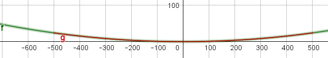
If the angle, $\theta$ is small we can make a reasonable approximation of the curve shape to a parabola. The down force is given by $\omega_{0}x$ because $x\approx s.$ The horizontal force is given by $T_{0}.$ So $$\frac{dy}{dx}=\frac{\omega_{0}x}{T_{0}}=\frac{x}{a}.$$ $$\int_{0}^{y}dy=\int_{0}^{x}\frac{x}{a}$$ $$y=\frac{x^{2}}{2a}=\frac{\omega_{0}x^{2}}{2T_{0}}$$ The sag, $h,$ is the value of $y$ at an attachment point and $x$ is the horizontal distance from the lowest curve point (now called the vertex) to the base of a support pole. Sometimes we see this equation written where $2x=L,$ the distance between poles. Then $$\frac{\omega_{0}\left(\frac{L}{2}\right)^{2}}{2T_{0}}=\frac{\omega_{0}L^{2}}{8T_{0}}.$$ Let's look at a graph.